Outlier Dip Trough Detection

[pjohnson1]

I am working on time series data and would like to detect these type of trough's in the graphs.   The y axis is network bandwidth and minimum value is 0.

I'm applying the base query time series to a DensityProbability model then with the following SPL for the Outlier chart:

| eval leftRange=mvindex(BoundaryRanges,0)
| eval rightRange=mvindex(BoundaryRanges,1)
| rex field=leftRange "Infinity:(?<lowerBound>[^:]*):"
| rex field=rightRange "(?<upperBound>[^:]*):Infinity"
| fields _time, 1/1/g1, lowerBound, upperBound, "IsOutlier(1/1/g1)", *

What approach can I take to detect the significant dip in the graph?

[tscroggins · Accepted solution]

@pjohnson1 

Are you fitting your model using stable data without outliers?

Here's an example you can recreate without data:

First, let's a define two macros to generate a bit of Gaussian noise:

# macros.conf

[norminv(3)]
args = p,u,s
definition = "exact($u$ + $s$ * if($p$ < 0.5, -1 * (sqrt(-2.0 * ln($p$)) - ((0.010328 * sqrt(-2.0 * ln($p$)) + 0.802853) * sqrt(-2.0 * ln($p$)) + 2.515517) / (((0.001308 * sqrt(-2.0 * ln($p$)) + 0.189269) * sqrt(-2.0 * ln($p$)) + 1.432788) * sqrt(-2.0 * ln($p$)) + 1.0)), (sqrt(-2.0 * ln(1 - $p$)) - ((0.010328 * sqrt(-2.0 * ln(1 - $p$)) + 0.802853) * sqrt(-2.0 * ln(1 - $p$)) + 2.515517) / (((0.001308 * sqrt(-2.0 * ln(1 - $p$)) + 0.189269) * sqrt(-2.0 * ln(1 - $p$)) + 1.432788) * sqrt(-2.0 * ln(1 - $p$)) + 1.0))))"
iseval = 1

[rand]
definition = "random()/2147483647"
iseval = 1

norminv(3) is similar to the Excel, Matlab, et al. norminv function and returns the inverse of the normal cumulative distribution function with a probability of p, a mean of u, and standard deviation of s. p must be greater than 0 and less than 1. The estimator is taken from Abramowitz and Stegun. More precise estimators can be taken from e.g. Odeh and Evans, but this is fine for toys like this.

rand() generates a random number between 0 and 1 using the known range of Splunk's random() function.

Next, let's generate some training data and fit it to a model:

| gentimes start=04/30/2021:00:00:00 end=05/01/2021:00:00:00 increment=1m 
| eval _time=starttime 
| fields + _time 
| eval x=`norminv("`rand()`*(0.9999999999999999-0.0000000000000001)+0.0000000000000001", 0.25, 0.05)`
| fit DensityFunction x into simple_gaussian_model

We can review the model parameters with the summary command:

| summary simple_gaussian_model

type	min	max	mean	std	cardinality	distance	other
Auto: Gaussian KDE	0.106517	0.386431	0.251574	0.042535	1440	metric: wasserstein, distance: 0.0010866394106055493	bandwidth: 0.009932847538368504, parameter size: 1440

Very close to our original mean of 0.25 and standard deviation of 0.05!

Finally, let's generate some test data and apply the model:

| gentimes start=05/01/2021:00:00:00 end=05/01/2021:09:00:00 increment=1m 
| eval _time=starttime 
| fields + _time 
| eval x=`norminv("`rand()`*(0.9999999999999999-0.0000000000000001)+0.0000000000000001", 0.25, 0.05)` 
| append 
    [| gentimes start=05/01/2021:09:00:00 end=05/01/2021:11:00:00 increment=1m 
    | eval _time=starttime 
    | fields + _time 
    | eval x=`norminv("`rand()`*(0.9999999999999999-0.0000000000000001)+0.0000000000000001", 0.01, 0.005)`] 
| append 
    [| gentimes start=05/01/2021:11:00:00 end=05/01/2021:12:00:00 increment=1m 
    | eval _time=starttime 
    | fields + _time 
    | eval x=`norminv("`rand()`*(0.9999999999999999-0.0000000000000001)+0.0000000000000001", 0.25, 0.05)`]
| apply simple_gaussian_model
| rex field=BoundaryRanges "-Infinity:(?<lcl>[^:]+)"
| rex field=BoundaryRanges "(?<ucl>[^:]+):Infinity"
| table _time x lcl ucl

 

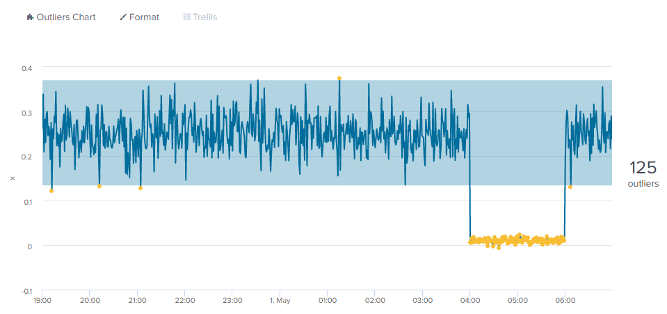
Very nice!

You can find the outliers directly--as you would in an alert search, for example--with a simple where command:

| apply simple_gaussian_model
| where 'IsOutlier(x)'==1.0
| table _time x

_time	x
2021-05-01 00:41:00	0.379067377
2021-05-01 02:54:00	0.411517318
2021-05-01 03:01:00	0.100776418
2021-05-01 07:18:00	0.131441104
2021-05-01 08:43:00	0.119352555
2021-05-01 08:49:00	0.379070878
2021-05-01 09:00:00	0.017377844
2021-05-01 09:01:00	0.013617436
2021-05-01 09:02:00	0.009148409
.	.
.	.
.	.

[pjohnson1]

Yes, I am fitting the data without outliers.

Initially I was using time slice buckets then fit with the by clause. This produced a range for each minute (I think), so the range kept changing.

| eval date_minutebin=strftime(_time, "%M")
| eval date_hour=strftime(_time, "%H")
| eval date_wday=strftime(_time, "%A")
| fit DensityFunction 1/1/g1 by "date_minutebin,date_hour,date_wday" into df_model threshold=0.05 dist=norm

For this specific case it was probably not needed, since I needed to look for outliers when the overall bandwidth was reduced (ie. high/low range for the whole data set).  Hopefully this makes sense.

As per your example if I kept it simple without the by clause, I get the desired result.

| fit DensityFunction 1/1/g1 into df_model dist=norm

For completeness - in my other data sets running the same fit parameters, is it possible to set lowerBound/lcl to zero since bandwidth cannot be a negative number? 

Thank you for explaining how to create the test data. I found that really neat!

[tscroggins]

@pjohnson1 

The dist=norm parameter tells the DensityFunction algorithm to use the normal distribution, which has bounds at -Infinity and +Infinity.

I used the default value (dist=auto), and the algorithm selected Gaussian kernel density estimation (dist=gaussian_kde).  I also constrained my mean and standard deviation in a way that would decrease the probability of test samples with values less than 0.

In practice, a normal distribution probably isn't the best fit for your data. We're not doing machine learning here so much as we are basic statistical analysis.

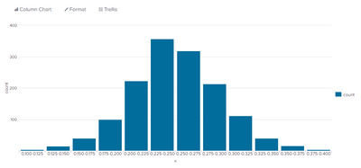
To see the shape of your data, the MLTK includes a histogram macro that works with the histogram visualization, but I prefer the chart command and the bar chart visualization. Just note that chart, bin, etc. produces duplicate bins when working with non-integral spans. I work around that bug with sort and dedup:

| gentimes start=04/30/2021:00:00:00 end=05/01/2021:00:00:00 increment=1m 
| eval _time=starttime 
| fields + _time 
| eval x=`norminv("`rand()`*(0.9999999999999999-0.0000000000000001)+0.0000000000000001", 0.25, 0.05)`
| chart count over x span=0.025
| sort - count
| dedup x
| sort x

My sample data is normally distributed as expected.

[pjohnson1]

This is what that data set look like.

Base query
| fit DensityFunction 1/1/g1 show_density=true
| bin 1/1/g1 bins=100
| stats count avg("ProbabilityDensity(1/1/g1)") as pd by 1/1/g1
| makecontinuous 1/1/g1
| sort 1/1/g1

For fit I have reset the value back to auto. dist=auto

For apply I have dropped the -  for the lcl value boundary range.

| apply 1/1/g1
| rex field=BoundaryRanges "Infinity:(?<lcl>[^:]+)"
| rex field=BoundaryRanges "(?<ucl>[^:]+):Infinity"
| table _time 1/1/g1 lcl ucl

The chart looks good now.

Thank you for the assistance.  It has been really helpful.